Checking for Solar Wind Charge Exchange(SWCX)
Last Updated:2023/06/22
This part follows the steps from these two papers (but somewhat simplified):
1.
Identifying XMM-Newton observations affected by solar wind charge exchange. Part I (Carter & Sembay 2008)
.
2.
Identifying XMM-Newton observations affected by solar wind charge exchange. Part II (Carter et al. 2011)
.
Better read them first, especially the first one.
Here are what I use for this tutorial:
Source: MCXC J0106.8+0103
Observation ID: 0762870601
SAS Version: 19.0.0
Python version: 3
csh is used
Everything you need in this tutorial is in:
swcx.zip
.
You work in the main folder swcx, there are several subfolders:
1. src - the source code is found here.
2. InputFiles - the folder in which the good ccd lists for mos1(goodccdlist_mos1.dat) and mos2(goodccdlist_mos2.dat) are put. This is created in
Anomalous CCD Check
.
3. products - the files created in this tutorial. They are put in the main folder if you create them successfully.
If you have already finished the last chapter and keep everything well. Then, you just need to copy the scripts in src to your current src folder.
Here are what you need in the main folder swcx. You should have them already if you follow the steps in the previous chapters. I already put them in the zip file.
1. mos1S001-gti.txt(fits) and mos2S002-gti.txt(fits). These files are for extraction of good time intervals common to mos1 and mos2.
2. the clean event list: mos1S001-clean.fits, mos2S002-clean.fits and pnS003-clean.fits. You need them for everything.
Basic ideas:
1. A "line" lightcurve (0.5-0.7, where SWCX is found), and a "continuum" lightcurve (2.5 - 5.0 keV, where SWCX is not found) binned in 1000 seconds are extracted, then make a scatter plot with x=continnum and y=line. A linear correlation is assumed in case of no SWCX (but sometimes scatter does not necessarily indicate SWCX). Reduced χ2 is derived using this equation:
Since y is the line lightcurves, I take σ as the error of y.
2. In the paper, it says "we computed the χ2 values for each individual lightcurve and calculate the ratio(R) between the line and continuum band χ2 values". I am not sure whether I get this right...I think x and y are reversed for step 1 and χ2 is re-calculated. But since σ is small for the continuum, this results in a big χ2, and the ratio is always smaller than 1...
Summing the above, I only provide a line-continuum scatter plot and the value of reduced χ2. I don't do exactly in the same way as the papers. They are more strict. If you read the paper, to determine whether SWCX exists is complicated, there are some exceptional cases where you cannot tell whether SWCX exists with the value of reduced χ2 and the ratio R, and there is no absolute threshold above which SWCX exists. Check the plot by eyes first anyway.
Detailed steps:
You just have to run the following and everything is done:
python3 src/swcx_script.py &
1. To combine the lightcurves of mos1 and mos2, the common good time interval is extracted first.
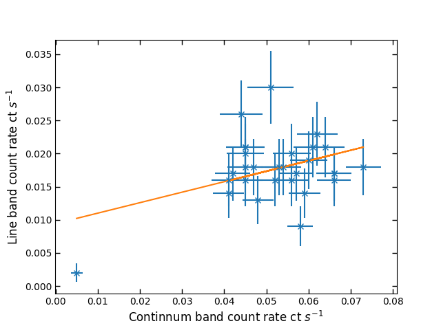 Fig.1. line-continnuum scatter plot with best-fit of mos1
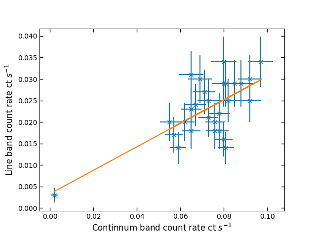 Fig.2. line-continnuum scatter plot with best-fit of mos2
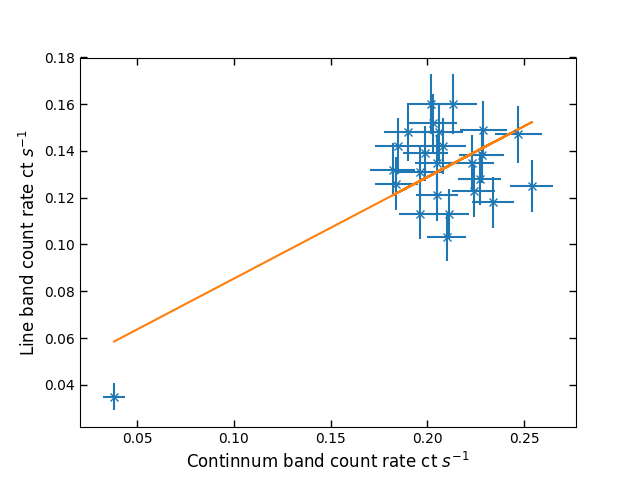 Fig.3. line-continnuum scatter plot with best-fit of pn
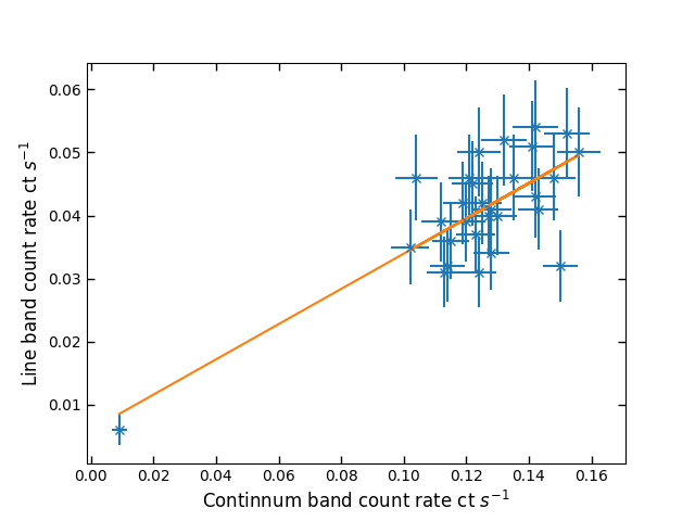 Fig.4. line-continnuum scatter plot with best-fit of combined mos1 and mos2
Here are the reduced χ2 found:

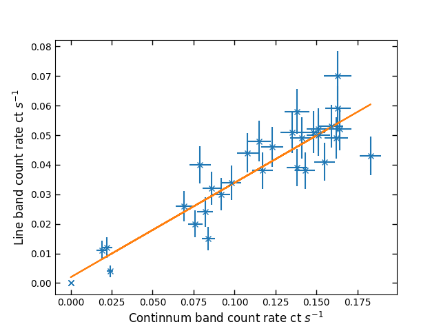 Fig.5. line-continnuum scatter plot with best-fit of pn(up,reduced χ2 = 2.2) and combined mos1+mos2(down,reduced χ2 = 1.9) of MCXC J0158.4-0146 (Obid: 0762870301)
Here are examples where SWCX are obvious.
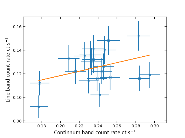
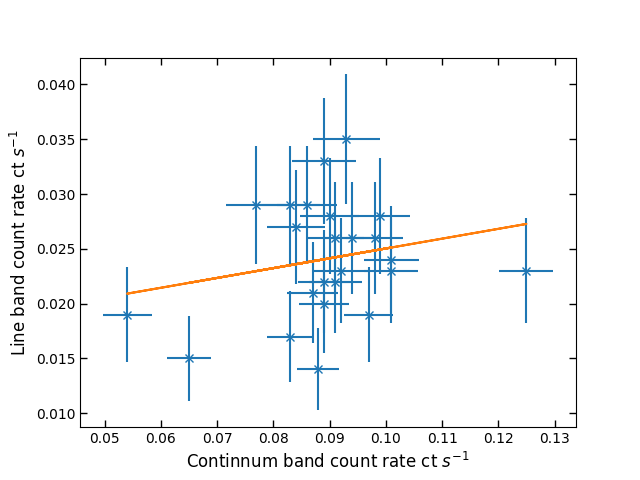 Fig.6. line-continnuum scatter plot with best-fit of pn(up,reduced χ2 = 1.7) and mos2(down,reduced χ2 = 1.3) of MCXC J0231.7-0451 (Obid: 0762870201)
So from the above example, you see the first example, MCXC J0158.4-0146, has got a good fit but a larger reduced χ2. It just depends on the error size ...
Sometimes it is really hard to decide whether SWCX exists and you don't want to go too deep spending too much time to find it out. For very contaminated sources, you can actually see clear solar line emissions in the spectrum (see fig.11 of the 2008 paper). If you think SWCX exists, you can include the emission lines in the spectral fit first, and check for the flux to see its strength first. We will talk more in
Spectral Fit
.